From smooth flow
to a singularity.
The same equations that help us understand air and water raise a surprisingly basic question: can a perfectly smooth flow develop infinite speed in finite time? OpenAI published a mathematical construction addressing that question. This project explores its concentrating flow with a numerical solver.
See the final continuationNavier–Stokes is a pervasive model of fluid flow
Navier–Stokes expresses Newton’s laws for a continuous fluid: motion changes as momentum is transported, pressure pushes, and viscosity smooths velocity differences. These equations underpin models of aircraft aerodynamics, weather, and blood flow.
The mathematical challenge is whether that smoothing always prevents a three-dimensional flow from losing its regularity. A singularity marks a limit of the mathematical description; it does not mean real water reaches infinite speed. Background ↗
OpenAI showed it can blow up under special forcing
On September 8, 2026, OpenAI released an analytical proof and a Lean formalization. The published theorem ↗ constructs a three-dimensional, incompressible flow that starts at rest: under a specially constructed external force that stays smooth, its peak speed becomes unbounded as a finite time approaches, while total kinetic energy remains bounded.
This is a specially forced counterexample. It establishes the breakdown alternatives C and D in Clay’s formulation ↗; it does not establish blowup for unforced Navier–Stokes or say that ordinary flows must become singular.
Here we run a simulation, which is not a proof
Here, AMReX / incflo advances velocity on fixed nested grids. We choose a target inspired by the proof and calculate the force needed to make it satisfy the discretized momentum equation. This manufactured solution lets us test whether the solver tracks the target and see how its geometry evolves.
Every run stops before the proposed singular time. A rising peak or a dramatic movie cannot establish infinite speed: grid spacing, timesteps, and the chosen force all affect the result. The useful evidence is how errors and resolved scales change under refinement. Numerical checks ↗
Completed October 2, 2026
The final finite continuation
The accepted 128³-base, five-level branch reaches t = 0.9975 at step 6,300. Its audited lineage contains 320 native states from exact rest, with 10,810,304 active cells and 2048³-equivalent spacing inside the finest cube.
The extension follows one grid-dependent trajectory. The latest resolution-tested candidate interval is t = 0.615808–0.629071; residual convergence and singularity formation remain unproven. Full numerical record →
Active solver cells
10,810,304
128³ base · outer bands · 2048³-equivalent core only
Saved frames from rest
320
Complete lineage · t = 0 to 0.9975
Endpoint peak speed
10.542
Model units · final continuation at t = 0.9975
What the final continuation shows
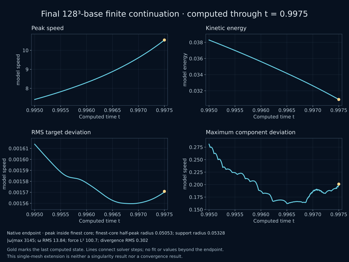
Computed solver-step diagnostics from t = 0.995 to 0.9975. Gold marks the last computed state; the lines contain no fit or projected values beyond the endpoint.
Scroll sideways to inspect all four continuation panels.
At t = 0.9975, peak speed is 10.5416, peak sampled vorticity is 3,144.97, and the half-peak support equivalent radius is 0.05328. The sampled divergence maximum is 153.53, and this single-mesh extension is neither a convergence result nor evidence of singularity formation.
How the fluid moves
The accepted Oliver parent and Mali continuation, from exact rest through t = 0.9975. All 320 audited states are included. Fixed x–y and x–z slices sit beside an isometric view of the same native field.
Fixed planes: y = 0 and z = 0. No vector arrows.
Loading the completed velocity movie.
Scroll sideways: x–y → x–z → isometric
Cameras, slice planes, and color scales stay fixed across all saved states. The 3D surfaces reconstruct native magnitudes for display; no intermediate times are invented. Use fullscreen or download the MP4 for the clearest view. Rendering details →
The force driving it
The applied force across the same 320 saved states and fixed planes as the velocity movie. Force uses its own fixed color scale and surface thresholds.
Fixed planes: y = 0 and z = 0. No vector arrows.
Loading the completed forcing movie.
Scroll sideways: x–y → x–z → isometric
The mesh beneath the motion
A 128³ base covers the full periodic box. Four fixed nested cubes refine the core, and 27 outer bands add resolution around the wider flow. The innermost cube reaches 2048³-equivalent spacing. The hierarchy stores 12,055,040 cells; 10,810,304 remain active after covered coarse cells are excluded.
x–y slice · z = 0

Isometric

Whole mesh · rotate
Scroll sideways: x–y → isometric → rotatable mesh
Central sections show actual active cell edges, including the irregular outer refinement. Outlines mark the central cubes. Covered coarse interiors are excluded.